The following equations describe a node in its most general sense. A node may contain :

• a pond ;
• several intakes or offtakes ;
• several upstream or downstream reaches.

The concepts and variables used at a node are describe in the following diagram :

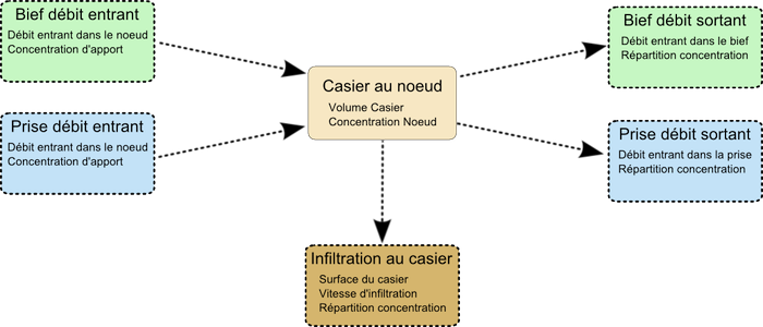
A pond is stored as a monotonous sequence of pairs (Surface, Elevation). The evaporation and the infiltration can be modelled with an evaporation rate $V_{ep}(t)$ and an infiltration rate $v_{inf}(Z_{nd})$,
$Z_{nd}$ being the water level in the pond.

The node gains or loses water through offtakes ($Q_p$) and reaches ($Q_b$).
Inflow is positive, whereas outflow is negative.

Reaches are given a time invariant flow direction according to their topology, which is :

• $s_{b}=1$ for inflow
• $s_{b}=-1$ for outflow

The discharge $Q_b$ is positive if it flows is in the same direction as the above topologic flow direction, and negative otherwise. The actual discharge is therefore given by : $s_{b}Q_{b}$

Inflow (positive discharge)

For upstream or downstream reaches with $s_{b}Q_{b}>0$ or offtakes with $Q_{p}>0$ there is a boundary condition for transported quality classes
$C$ which is the concentration incoming.

Outflow (negative discharge)

Reaches

For upstream or downstream reaches with $s_{b}Q_{b}<0$ , we have
$C_{b}=k_{b}C_{nd}$ .

Offtakes

For offtakes with $Q_{p}<0$ , we have $C_{p}=k_{p}C_{nd}$ ($k_{p}$ is describe later).

Infiltration at the node

We have $C_{\mathit{inf}}=k_{\mathit{inf}}C_{\mathit{nd}}$ and
$Q_{\mathit{inf}}=S_{\mathit{cas}}v_{\mathit{inf}}$ where :
$S_{cas}$ is the pond area, $v_{inf}$ is the infiltration rate and
$C_{\mathit{nd}}$ is the node concentration.

Storage flow in the pond

The pond is connected to the node, and the concentrations at the node and the pond are the same.
The stored amount of a class in the pond is :
$m_{\mathit{Cas}}=V_{\mathit{Cas}}C_{\mathit{nd}}$ and the flow in or out is :
$Q_{\mathit{cas}}=S_{\mathit{cas}}\frac{\mathit{dZ}_{\mathit{nd}}}{\mathit{dt}}$.

Mass balance at the node

The mass balance equation for a quality class in the node is :

$\frac{\mathit{dm}_{\mathit{nd}}}{\mathit{dt}}=\sum_{s_{b}Q_{b}>0}C_{b}s_{b}Q_{b}+\sum_{s_{b}Q_{b}<0}k_{b}s_{b}Q_{b}C_{\mathit{nd}}$
$+\sum_{Q_{p}>0}C_{p}Q_{p}+\sum_{Q_{p}<0}k_{p}Q_{p}C_{\mathit{nd}}-k_{\mathit{inf}}S_{\mathit{cas}}C_{\mathit{nd}}v_{\mathit{inf}}+V_{\mathit{Cas}}E(t,C_{\mathit{nd}})$

With $\frac{\mathit{dm}_{\mathit{nd}}}{\mathit{dt}}=\frac{d\left(C_{\mathit{nd}}V_{\mathit{cas}}\right)}{\mathit{dt}}=\frac{dV_{\mathit{cas}}}{\mathit{dt}}C_{\mathit{nd}}+\frac{dC_{\mathit{nd}}}{\mathit{dt}}V_{\mathit{cas}}$,
the equation gives :

$\sum _{s_{b}Q_{b}>0}C_{b}s_{b}Q_{b}+\sum _{Q_{p}>0}C_{p}Q_{p}+V_{\mathit{Cas}}\left(E(t,C_{\mathit{nd}})-\frac{\mathit{dC}_{\mathit{nd}}}{\mathit{dt}}\right)$
$+C_{\mathit{nd}}\left[\sum _{s_{b}Q_{b}<0}k_{b}s_{b}Q_{b}+\sum _{Q_{p}<0}k_{p}Q_{p}-k_{\mathit{inf}}S_{\mathit{cas}}v_{\mathit{inf}}-\frac{\mathit{dV}_{\mathit{cas}}}{\mathit{dt}}\right]=0$

where $S_{cas}$, $V_{cas}$ , $Z_{nd}$ are the area, volume and water level of the pond.

Distribution coefficient $k$

3 cases are considered for the outflow distribution coefficients :

Outflows are homogeneous

All k are 1 : whatever the evolution of flow and contentrations, the mass balance equation is used to compute the concentration in outflows.

Outflows are heterogeneous and the node contains a pond

The concentration entering or leaving the pond ensures mass balance at the node.

Outflows are heterogeneous and the node does not contain a pond

Some distribution coefficients must be adjusted (while remaining positive) to maintain the mass balance condition.

The distribution coefficients are given by the user for each offtake and reach and for infiltration, and can be defined as fix ($b_i=0$) or adjustable ($b_i=1$) to ensure continuity at the node.

An adjustement coefficient $k_a$ for the node is computed and the distribution coefficients become :${k_{a}}^{b_{i}}k_{i}$. Therefore, a fix coefficient ($b_i=0$) is not changed ${k_{a}}^{b_{i}}k_{i}=k_{i}$ whereas an adjustable coefficient becomes ${k_{a}}^{b_{i}}k_{i}=k_{a}k_{i}$.

The new mass balance equation is :

$\sum _{Q_{i}>0}C_{i}Q_{i}+C_{\mathit{nd}}\left[\sum _{Q_{i}<0,b_{i}=0}k_{i}Q_{i}+k_{a}\sum _{Q_{i}<0,b_{i}=1}k_{i}Q_{i}\right]=0$

$k_{a}=-{\frac{\frac{1}{C_{\mathit{nd}}}\sum _{Q_{i}>0}C_{i}Q_{i}+\sum _{Q_{i}<0,b_{i}=0}k_{i}Q_{i}}{\sum _{Q_{i}<0,b_{i}=1}k_{i}Q_{i}}}$

where ${C_{\mathit{nd}}}$ is the node concentration given by

$C_{\mathit{nd}}=\frac{\sum _{Q_{i}>0}C_{i}Q_{i}}{\sum _{Q_{i}>0}Q_{i}}$

The equation for $k_a$ is :

$k_{a}=-{\frac{\sum _{Q_{i}>0}Q_{i}+\sum _{Q_{i}<0,b_{i}=0}k_{i}Q_{i}}{\sum _{Q_{i}<0,b_{i}=1}k_{i}Q_{i}}}$

$k_{a}=-{\frac{\left(\sum _{s_{b}Q_{b}>0}s_{b}Q_{b}+\sum _{Q_{p}>0}Q_{p}\right)+\left(\sum _{s_{b}Q_{b}<0,b_{b}=0}k_{b}s_{b}Q_{b}+\sum _{Q_{p}<0,b_{p}=0}k_{p}Q_{p}\right)}{\sum _{s_{b}Q_{b}<0,b_{b}=1}k_{b}s_{b}Q_{b}+\sum _{Q_{p}<0,b_{p}=1}k_{p}Q_{p}}}$

The final mass balance equation is :

$\sum _{s_{b}Q_{b}>0}C_{b}s_{b}Q_{b}+\sum _{Q_{p}>0}C_{p}Q_{p}+C_{\mathit{nd}}\left(\sum _{s_{b}Q_{b}<0}{k_{a}}^{b_{b}}k_{b}s_{b}Q_{b}+\sum _{Q_{p}<0}{k_{a}}^{b_{p}}k_{p}Q_{p}\right)=0$

or

$\sum _{s_{b}Q_{b}>0}C_{b}s_{b}Q_{b}+\sum _{Q_{p}>0}C_{p}Q_{p}$
$+C_{\mathit{nd}}\left[\sum _{s_{b}Q_{b}<0,b_{b}=0}k_{b}s_{b}Q_{b}+\sum _{Q_{p}<0,b_{p}=0}k_{p}Q_{p}+k_{a}\left(\sum _{s_{b}Q_{b}<0,b_{b}=1}k_{b}s_{b}Q_{b}+\sum _{Q_{p}<0,b_{p}=1}k_{p}Q_{p}\right)\right]=0$